A drying-tunnel zone passed every test on the day it went in. The activation class was right, the cold loop resistance landed cleanly inside the panel's window, and a heat-gun check produced a sharp alarm. Two years later the same zone nuisance-trips on the benign heat of every shift start-up — peaks it used to ride out without complaint. Nothing is corroded. Nothing is wet. The terminations are still tight. The cable has simply been heated and cooled a few thousand times — and it no longer returns to exactly where it started.
This note is about that slow walk: what a single heat-cool cycle does to the compound, insulation and terminations, why the small amount that does not recover each time accumulates, and how to specify and verify a cable so the cycles do not quietly drift the activation point out of band. Cycling fatigue is one of the four aging families surveyed in the thermal sensor cable engineering reference; here it gets the dedicated treatment that overview pointed to. It is not about where to physically position a cable next to a pulsing heater — that standoff-and-jacket problem is the subject of the cyclic-duty placement playbook — nor is it conductor oxidation, the chemistry-driven mechanism in the rapid-oxidation note. Cycling fatigue is mechanical and thermal rather than chemical, and it is counted in cycles, not years.
What One Heat-Cool Cycle Does
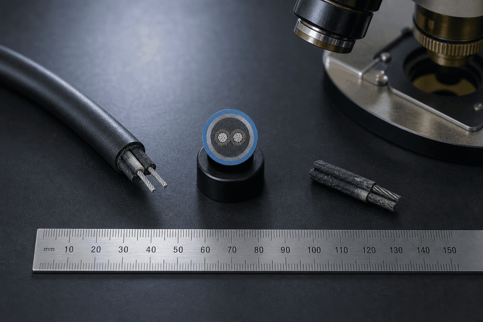
Each time the cable warms toward its activation region and cools back, three layers move at once — and they move by different amounts and at different rates. That mismatch is the whole story.
The active sensing material softens as it approaches the activation point and stiffens again on cooling. Each pass through that softening region lets the polymer chains relax slightly into a new arrangement. Most of it recovers; a fraction sets. That fraction is exactly the property that fixes where the resistance collapses, so it is the layer whose drift the panel eventually reads.
The polymer wall expands and contracts with every swing, and it does so at a different coefficient than the compound and the conductors it surrounds. Over many cycles that differential strain works the interfaces between layers — the first visible signs are micro-cracking and a gradual loss of flexibility long before the jacket fails an IP test.
A lug or crimp that never moves stays low-resistance for decades, provided it was clean and tight to begin with. One that is cycled grows and shrinks against the hardware it is clamped into, and the micro-movement slowly polishes and unseats the contact. The result is a creeping rise in contact resistance that stacks onto the loop total — the same direction as a loosening joint, but driven by the cycles rather than time.
On a single cycle none of this is measurable. The compound returns, the jacket relaxes, the joint reseats. The mechanism only matters because the cable does it again, and again, and the tiny residue from each pass does not undo itself.
Why the Drift Accumulates — Recovery Is Never Complete
The reason an activation point moves at all is that the recovery on the cooling half of the cycle is not a perfect mirror of the heating half. The compound returns to almost its original state, with a small hysteresis — a little of the change is retained. Run one cycle and the retained part is far too small to find. Run a thousand cycles through a large swing and those retained parts have summed into a shift big enough to read as a few kelvin of activation drift.
That is why the cable behaves as if it “remembers”: it is carrying the accumulated residue of every cycle it has been through. Two cables stamped with the same activation class can age completely differently on this axis — one in a stable tray that never swings, one beside a short-cycle process — and after a couple of years they no longer trip at the same temperature, even though both were identical on the data sheet. This is the cycling-fatigue slice of the broader picture in which two cables stamped 105 °C can drift apart by 20 K over a deployment lifetime, with oxidation, moisture and dielectric aging each adding their own contribution on top.
Counted in Cycles and Swing Amplitude, Not Calendar Years
The single most common mistake is to treat cycling life as a number of years. It is not. Two route variables set the severity, and calendar time only matters through them: the number of cycles imposed, and how large each temperature swing is relative to the activation point. A small swing well below activation barely fatigues the compound no matter how often it repeats; a swing that drives the compound up into its softening region does real work on every pass.
| Route character | Cycling-fatigue severity |
|---|---|
| Quiet tray, small swings | Ambient drifts a few degrees day to night and the cable stays far below activation. Swing amplitude is small, so even years of daily cycles do little measurable work. Cycling drift is rarely the life-limiting mechanism here. |
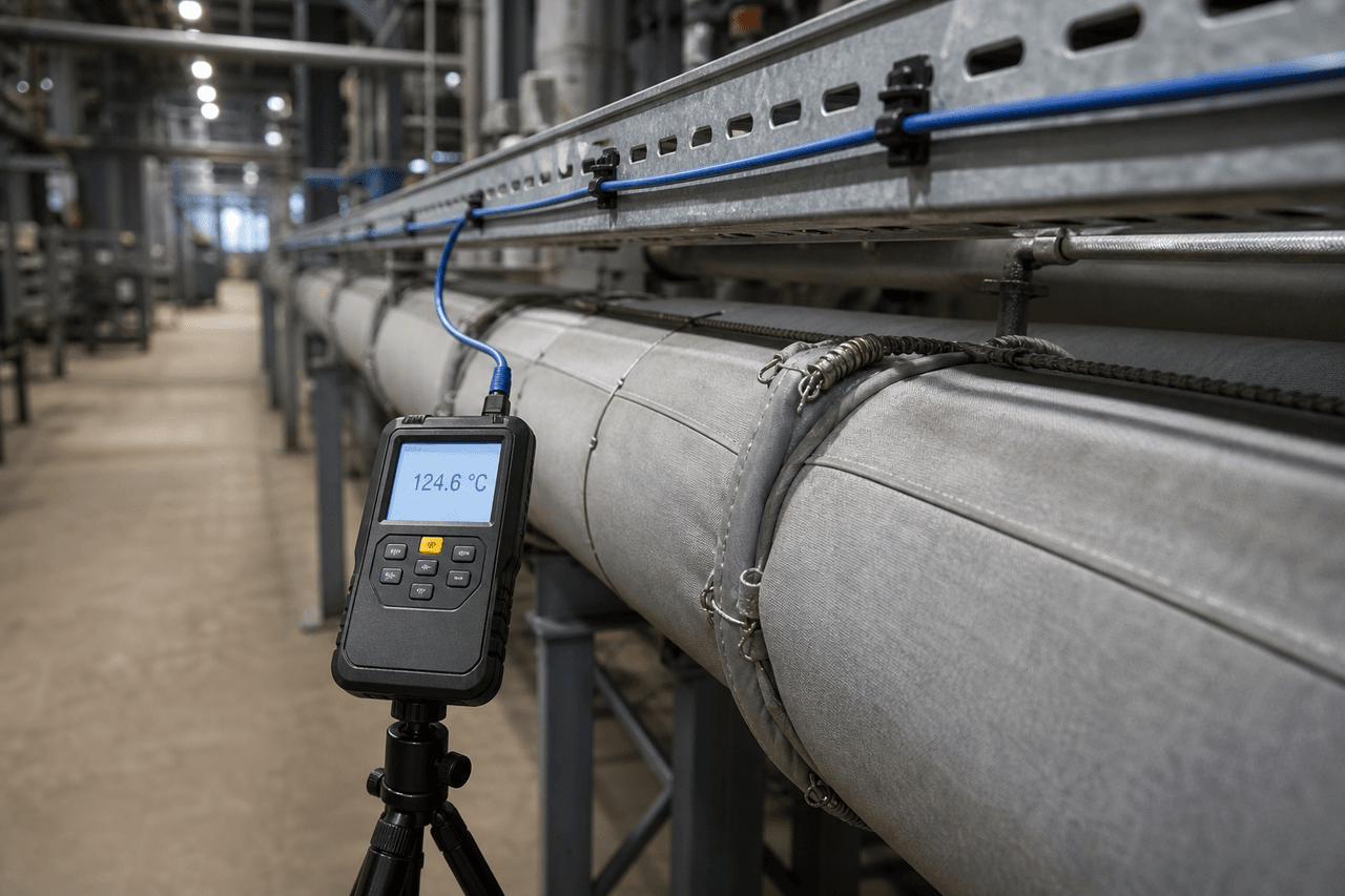
| Daily process cycle, moderate swings | An oven, dryer or batch process heats the zone toward — but not into — the activation region once or a few times a day. The compound is worked but not driven through its softening peak; drift is slow and shows up over years, worth a periodic re-check. |
| Short-cycle or PWM hot zone, large swings | A pulsed heater, drive or short-cycle element swings the cable close to its activation point many times per hour. Both inputs are high at once — many cycles and a large amplitude — so drift accumulates fastest and the order-of-magnitude marker of a thousand cycles is reached soonest. |
The thousand-cycle figure that gives this kind of fatigue its reputation is best read as an order-of-magnitude marker for where drift becomes worth measuring on an aggressive route — not a cliff the cable falls off at cycle 1,001. Where it lands for a given construction depends on the compound chemistry and the swing it is driven through, which is why the cycle profile belongs on the specification rather than being inferred from a peak-temperature rating alone.
Estimating Cycling Life Without Over-Promising
Because the mechanism is cumulative and chemistry-dependent, the honest way to estimate cycling life is relative, not absolute. Two cables, or two routes, can be ranked against each other with confidence; converting that into a single guaranteed hour or cycle figure for a specific install is where the estimate gets fragile, because it depends on the exact compound, the real swing the route imposes, and how close the working peak sits to the activation point.
Two inputs drive cycling severity:

  cycles imposed      =  cycles per day  ×  service days
  work per cycle      ↑  as the swing peak approaches the activation point

Severity rises with BOTH. A route can be high-cycle/low-amplitude
(many gentle swings) or low-cycle/high-amplitude (few hard swings);
the punishing case is high on both at once.
What this means in practice is that a cable can be qualified for a cyclic-duty route by testing it under a representative cycle and comparing the drift to a budget, rather than by quoting a lifetime. The tolerance band a buyer writes on the specification should be set with room for this drift built in, the same way it should leave room for oxidation and dielectric aging — the reasoning behind sizing that band sits in the activation temperature selection note, and the broader point that a data-sheet band describes the cable as-shipped rather than after years in service is made in the custom activation tolerance note. Cycling fatigue is one of the reasons the as-shipped band and the in-service band are not the same number.
Specifying a Cable That Survives the Cycles
The specification side of cycling fatigue comes down to one habit most data sheets do not prompt for: describe the cycle, not just the peak. A cable rated for a 150 °C peak says nothing about how it behaves swinging to that peak twenty times a day. Putting the cycle profile on the RFQ turns an assumption into a requirement the supplier can match.
Duty profile: state peak temperature, valley temperature, cycle period and
approximate cycles per day for the route (not just a steady ambient).
Cycling data: request activation-drift results under a representative thermal
cycle for the supplied construction, with the cycle count tested.
Headroom: confirm the working swing peak stays below the activation point with
margin, so the compound is not driven through its softening region each cycle.
Jacket: select for repeated flex and thermal movement, not peak temperature alone.
Three levers follow from that profile. Leave headroom between the working swing and the activation point, so the compound spends most of each cycle below its softening region rather than inside it. Choose a jacket and insulation rated for repeated thermal movement and flex life, not only for a peak number — the trade-offs between silicone, fluoropolymer and fiberglass on exactly that axis are in the jacket and insulation material notes. And derate the placement: keeping the cable off the heater's normal radiant peak shrinks the swing it sees, which is the most direct way to reduce the work done per cycle. The placement geometry that achieves that — standoff, shielding and route — is the cyclic-duty placement playbook; the point here is that placement and specification together set how hard each cycle hits.
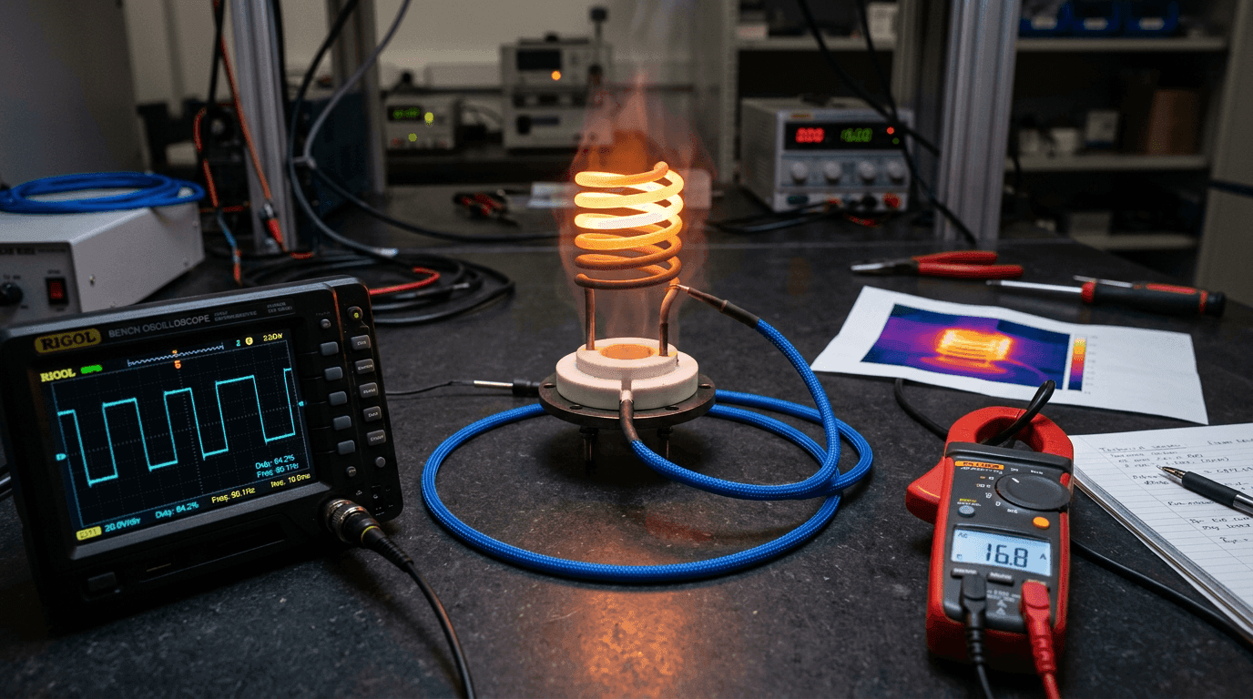
Verifying — Bench Cycling and the Drift Baseline
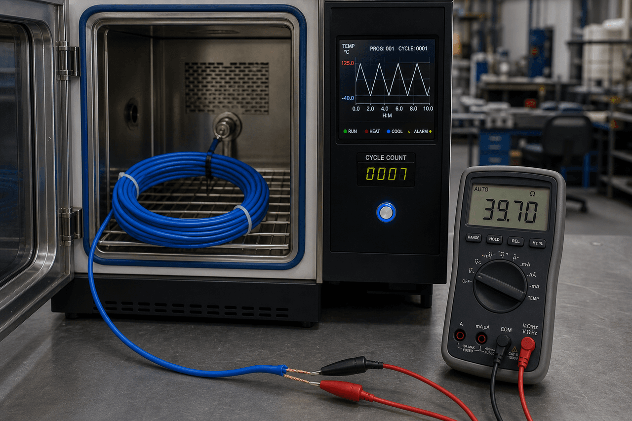
Cycling fatigue is one of the few aging mechanisms that is straightforward to reproduce on a bench, because the cycle is exactly what you can repeat on demand. A controlled-temperature chamber or oil bath ramped between the route's valley and peak, with the activation point and loop resistance measured every so many cycles, turns “it might drift” into a curve you can read — and lets two constructions be ranked under the same cycle before either is committed to a project.
In the field, the equivalent discipline is the baseline — with one caveat about what an installed run lets you re-measure. The cold loop resistance and insulation resistance recorded at commissioning, while the cable is new, can be re-checked for the life of the loop without disturbing it; the activation point usually cannot, because on a one-shot LHD construction the test that confirms it is the event itself. Activation drift is tracked instead on a retained or same-batch sample under bench cycling, while the installed loop is watched through its resistance trend:
A loop resistance that creeps up across re-checks over months points to cumulative aging in the conductor path and terminations — the contact-fretting layer of cycling fatigue, or another slow mechanism. On the sample bench the matching signature is the activation point edging off its first-cycle value, the compound layer of the same fatigue. Either way it is what the baseline exists to catch, early enough to plan a replacement rather than discover a missed alarm.
A reading that jumps rather than drifts is a discrete fault — a wet joint, a crush, a termination that has let go — not fatigue. Telling a slow trend apart from a step, and a real activation apart from either, uses the loop-resistance and insulation-resistance readings of the field-diagnosis sequence.
Recording that commissioning figure costs a few minutes and is the difference between watching cycling drift arrive and being surprised by it. On a quiet route it may never move; on a short-cycle hot zone it is the measurement that earns its keep.
A thermal sensor cable does not fail on a cyclic-duty route so much as it slowly forgets where its activation point was. Each heat-cool cycle leaves a residue the cable never fully sheds, and a few thousand of them add up to drift the panel eventually reads. The defence is not a tougher peak rating — it is specifying the cycle the cable will live in, leaving headroom so each swing does less work, and recording a baseline so the slow walk is something you measure rather than something that catches you.
FAQ — Thermal Sensor Cable Cycling Fatigue
What is thermal cycling fatigue in a thermal sensor cable?
Thermal cycling fatigue is the slow, cumulative change a thermal sensor cable undergoes when it is heated toward its activation region and cooled back many times. The compound, insulation, jacket and terminations each recover most of that movement every cycle but never all of it, and over hundreds to thousands of cycles the small retained fractions add up. The visible result is drift in the activation point — the cable still works, but no longer trips at exactly the temperature it did when new. Unlike oxidation or moisture ingress, cycling fatigue is mechanical and thermal rather than chemical, and it is driven by the number of cycles and the size of the temperature swing, not by calendar time alone.
After how many cycles does a thermal sensor cable's activation point drift?
There is no single cycle count that applies to every cable: the drift depends on how many cycles the route imposes and how large each temperature swing is. A cable in a quiet tray that barely warms can run for years with no measurable cycling drift, while one beside a short-cycle PWM heater that swings close to its activation point on every pulse accumulates drift far faster, because the compound is repeatedly driven through the softening region where the permanent change per cycle is largest. The often-quoted figure of around a thousand cycles is a useful order-of-magnitude marker for where drift becomes worth measuring on an aggressive route, not a guaranteed life. The dependable approach is to treat cycle count and swing amplitude as the two inputs, ask the supplier for cycle-test data on the specific construction, and re-measure against the commissioning baseline rather than assuming a fixed number.
How do you specify a thermal sensor cable for a cyclic-duty route?
Specifying for cyclic duty starts by describing the cycle the cable will live in, because that is the input a supplier needs and the figure most data sheets never ask for. State the peak temperature, the valley it returns to, the cycle period and the approximate cycles per day or per year, so the construction can be matched to the duty rather than to a single steady ambient. From there, three levers help: choose a jacket and insulation rated for repeated flex and thermal movement rather than only a peak temperature, leave headroom between the working swing and the activation point so the compound is not driven through its softening region on every cycle, and place the cable to see the threat without sitting in the heater's normal radiant peak. The placement side of that — standoff distance and jacket choice next to a pulsing heater — is a separate exercise covered on its own. The specification side is simply making the cycle profile an explicit line on the RFQ instead of an assumption.
How do you detect cycling drift before it causes a missed alarm or a nuisance trip?
Cycling drift is detectable because it is gradual and repeatable, which means a baseline turns it into something you can watch. Record the cold loop resistance and insulation resistance at commissioning, while the cable is new, and keep those figures. On a cyclic-duty route, re-checking them periodically will show a slow trend long before it becomes a missed alarm or a nuisance trip. The activation point itself usually cannot be re-confirmed on an installed run — on a one-shot LHD construction the test is the event — so activation drift is tracked on a retained or same-batch sample under bench cycling instead. A reading that creeps steadily in one direction points to cumulative aging such as cycling fatigue; a sudden step points to a discrete fault such as a wet joint or a crush, which is separated from slow drift using the same loop-resistance and insulation-resistance readings as the field-diagnosis sequence.